Image compression using Discrete cosine transforms.

This post first appeared on PhotoElectricChefs.

The internet has grown to connect a very large user base in recent times, but bandwidth still remains limited. Images take up a large amount of bandwidth, hence we make use of different image compression methods. One famous format is JPEG (Joint Photographic Experts Group), a widely accepted standard, which uses Discrete Cosine Transforms (DCT) for compression. In this post we will try to understand the simple idea behind the DCT.

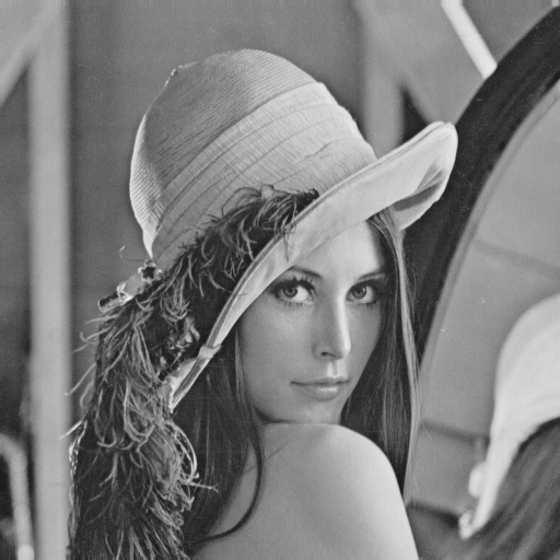
For the demo I will be using Octave (an equivalent of Matlab), and the following 512x512 image:

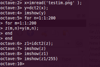
The code for understanding DCT is fairly simple.

• The first line reads the image into the matrix ‘x’. The image can now be imagined as a matrix of 512 rows and 512 columns, where each value of the matrix corresponds to the brightness of that part of the picture. For example, the eyes in the image may correspond to the location [260, 256]. The matrix value at this address is 0, indicating completely black (on a scale of 255, where 255 is white). If the picture was a colour image, each pixel would have three values, its red, green and blue intensities. This is referred to as a 3-channel image.
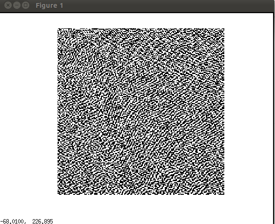
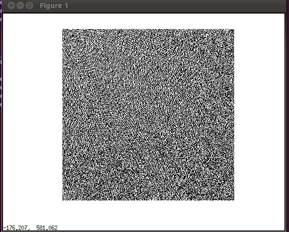
• Next we find the DCT of this image and store it in ‘y’. Remember that the DCT is not a one-to-one mapping like the case above: each matrix entry does not refer to one pixel of the picture. Instead the entries are the weights of different patterns that together make up the whole image. Not going much into the theory, let’s move on.
• The next 5 lines of code take a part of the matrix ‘y’ and save it into matrix ‘z’. Here only 200x200 elements of ‘y’ are saved in ‘z’. The plots of ‘y’ and ‘z’ are shown later. This operation is similar to cropping the image.
• Now we find the inverse DCT of the matrix ‘z’. This should give us the image back, but it will not. A scaling factor of around 255 is required, either multiply or divide, play around to find the correct one. Divide works for me.
• Hence the line: imshow(z1/255).

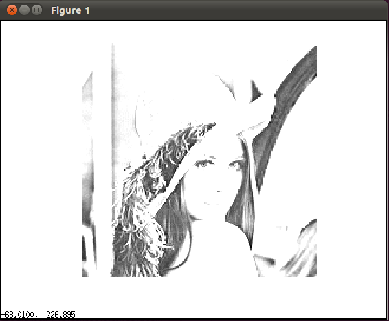
The resulting image is shown above. Now to understand what we actually did, we have to look at the details of the image.

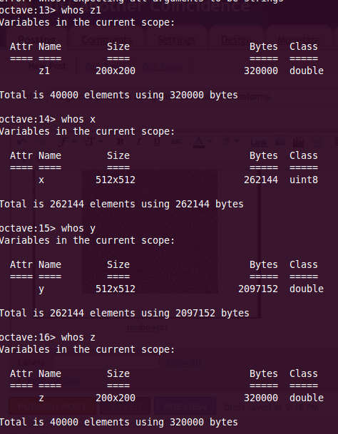
Just type in “whos z1” (without quotes) in your main terminal and you will see that the resulting image is 200x200. Not only has the image been resized, but the important point is that we recovered the complete image with only 200x200 values of the DCT. This is what we mean by energy compaction, where most of the image data is stored in the first few elements of the matrix. So instead of having 512x512 values, where each pixel is needed to define the picture, we have converted that to a 200x200 matrix where the first few entries describe the overall brightness of the whole picture, and the rest add the finer detail on top of it.

Hope this post has made you understand and appreciate image processing, and mainly maths. Comments are welcome! :)